Getting Started
Installing Platypus
To install the latest version of Platypus, run the following commands.
pip install -U build setuptools
git clone https://github.com/Project-Platypus/Platypus.git
cd Platypus
python -m build
A Simple Example
As an initial example, we will solve the well-known two objective DTLZ2 problem using the NSGA-II algorithm:
from platypus import NSGAII, DTLZ2

# Select the problem
problem = DTLZ2()

# Create the optimization algorithm.
algorithm = NSGAII(problem)

# Optimize the problem using 10,000 function evaluations.
algorithm.run(10000)

# Display the results.
for solution in algorithm.result:
    print(solution.objectives)
The output shows on each line the objectives for a Pareto optimal solution:
[1.00289403128, 6.63772921439e-05]
[0.000320076737668, 1.00499316652]
[1.00289403128, 6.63772921439e-05]
[0.705383878891, 0.712701387377]
[0.961083112366, 0.285860932437]
[0.729124908607, 0.688608373855]
...
If matplotlib is available, we can also plot the results. Note that matplotlib must be installed separately. Running the following code
from platypus import NSGAII, DTLZ2
import matplotlib.pyplot as plt

# Select the problem.
problem = DTLZ2()

# Create the optimization algorithm.
algorithm = NSGAII(problem)

# Optimize the problem using 10,000 function evaluations
algorithm.run(10000)

# Plot the results using matplotlib
plt.scatter([s.objectives[0] for s in algorithm.result],
            [s.objectives[1] for s in algorithm.result])
plt.xlim([0, 1.1])
plt.ylim([0, 1.1])
plt.xlabel("$f_1(x)$")
plt.ylabel("$f_2(x)$")
plt.show()
produce a plot similar to:
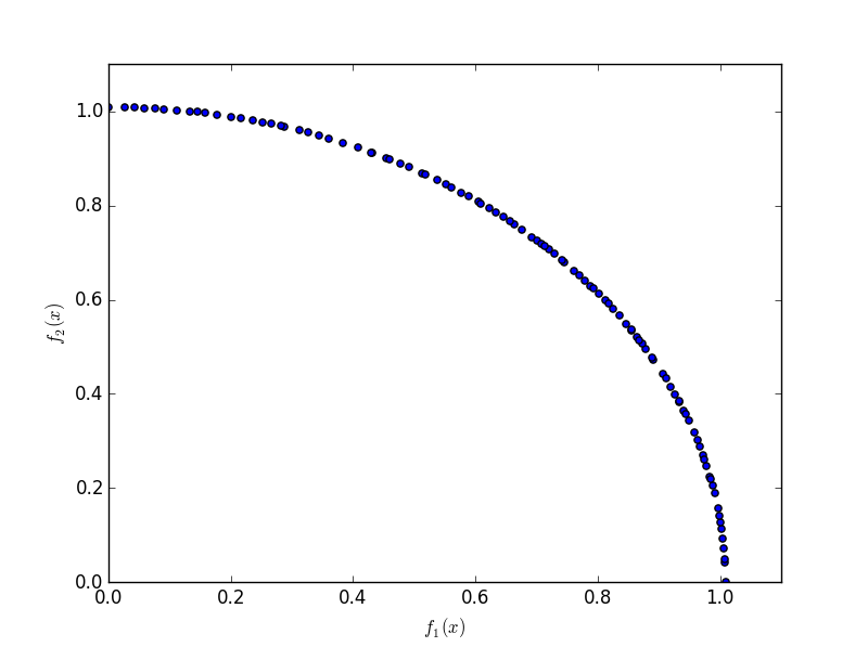
Note that we did not need to specify many settings when constructing NSGA-II. For any options not specified by the user, Platypus supplies the appropriate settings using best practices. In this example, Platypus inspected the problem definition to determine that the DTLZ2 problem consists of real-valued decision variables and selected the Simulated Binary Crossover (SBX) and Polynomial Mutation (PM) operators. One can easily switch to using different operators, such as Parent-Centric Crossover (PCX):
from platypus import NSGAII, DTLZ2, PCX

problem = DTLZ2()

algorithm = NSGAII(problem, variator=PCX())
algorithm.run(10000)
Defining Unconstrained Problems
There are several ways to define problems in Platypus, but all revolve around
the Problem class. For unconstrained problems, the problem is defined
by a function that accepts a single argument, a list of decision variables,
and returns a list of objective values. For example, the bi-objective,
Schaffer problem, defined by
![\text{minimize } (x^2, (x-2)^2) \text{ for } x \in [-10, 10]](_images/math/e20ef2c1d739f6b8cb6bd8c619914afdcb203016.png)
can be programmed as follows:
from platypus import NSGAII, Problem, Real

def schaffer(x):
    return [x[0]**2, (x[0]-2)**2]

problem = Problem(1, 2)
problem.types[:] = Real(-10, 10)
problem.function = schaffer

algorithm = NSGAII(problem)
algorithm.run(10000)
When creating the Problem class, we provide two arguments: the number
if decision variables, 1, and the number of objectives, 2. Next, we
specify the types of the decision variables. In this case, we use a real-valued
variable bounded between -10 and 10. Finally, we define the function for
evaluating the problem.
Tip: The notation problem.types[:] is a shorthand way to assign all
decision variables to the same type. This is using Python’s slice notation.
You can also assign the type of a single decision variable, such as
problem.types[0], or any subset, such as problem.types[1:].
An equivalent but more reusable way to define this problem is extending the
Problem class. The types are defined in the __init__ method, and the
actual evaluation is performed in the evaluate method.
from platypus import NSGAII, Problem, Real

class Schaffer(Problem):

    def __init__(self):
        super().__init__(1, 2)
        self.types[:] = Real(-10, 10)

    def evaluate(self, solution):
        x = solution.variables[:]
        solution.objectives[:] = [x[0]**2, (x[0]-2)**2]

algorithm = NSGAII(Schaffer())
algorithm.run(10000)
Defining Constrained Problems
Constrained problems are defined similarly, but must provide two additional pieces of information. First, they must compute the constraint value (or values if the problem defines more than one constraint). Second, they must specify when constraint is feasible and infeasible. To demonstrate this, we will use the Belegundu problem, defined by:

This problem has two inequality constraints. We first simplify the constraints by moving the constant to the left of the inequality. The resulting formulation is:

Then, we program this problem within Platypus as follows:
from platypus import NSGAII, Problem, Real

def belegundu(vars):
    x = vars[0]
    y = vars[1]
    return [-2*x + y, 2*x + y], [-x + y - 1, x + y - 7]

problem = Problem(2, 2, 2)
problem.types[:] = [Real(0, 5), Real(0, 3)]
problem.constraints[:] = "<=0"
problem.function = belegundu

algorithm = NSGAII(problem)
algorithm.run(10000)
First, we call Problem(2, 2, 2) to create a problem with two decision
variables, two objectives, and two constraints, respectively. Next, we set the
decision variable types and the constraint feasibility criteria. The constraint
feasibility criteria is specified as the string "<=0", meaning a
solution is feasible if the constraint values are less than or equal to zero.
Platypus is flexible in how constraints are defined, and can include inequality
and equality constraints such as ">=0", "==0", or "!=5". Finally,
we set the evaluation function. Note how the belegundu function returns
a tuple (two lists) for the objectives and constraints.
The final population could contain infeasible and dominated solutions if the
number of function evaluations was insufficient (e.g. algorithm.Run(100)).
In this case we would need to filter out the infeasible solutions:
feasible_solutions = [s for s in algorithm.result if s.feasible]
We could also get only the non-dominated solutions:
nondominated_solutions = nondominated(algorithm.result)
Alternatively, we can develop a reusable class for this problem by extending
the Problem class. Like before, we move the type and constraint
declarations to the __init__ method and assign the solution’s
constraints attribute in the evaluate method.
from platypus import NSGAII, Problem, Real

class Belegundu(Problem):

    def __init__(self):
        super().__init__(2, 2, 2)
        self.types[:] = [Real(0, 5), Real(0, 3)]
        self.constraints[:] = "<=0"

    def evaluate(self, solution):
        x = solution.variables[0]
        y = solution.variables[1]
        solution.objectives[:] = [-2*x + y, 2*x + y]
        solution.constraints[:] = [-x + y - 1, x + y - 7]

algorithm = NSGAII(Belegundu())
algorithm.run(10000)
In these examples, we have assumed that the objectives are being minimized.
Platypus is flexible and allows the optimization direction to be changed per
objective by setting the directions attribute. For example:
problem.directions[:] = Problem.MAXIMIZE