Experimenter

There are several common scenarios encountered when experimenting with MOEAs:

1. Testing a new algorithm against many test problems
2. Comparing the performance of many algorithms across one or more problems
3. Testing the effects of different parameters

Platypus provides the experimenter module with convenient routines for performing these kinds of experiments. Furthermore, the experimenter methods all support parallelization.

Basic Use

Suppose we want to compare NSGA-II and NSGA-III on the DTLZ2 problem. In general, you will want to run each algorithm several times on the problem with different random number generator seeds. Instead of having to write many for loops to run each algorithm for every seed, we can use the experiment function. The experiment function accepts a list of algorithms, a list of problems, and several other arguments that configure the experiment, such as the number of seeds and number of function evaluations. It then evaluates every algorithm against every problem and returns the data in a JSON-like dictionary.

Afterwards, we can use the calculate function to calculate one or more performance indicators for the results. The result is another JSON-like dictionary storing the numeric indicator values. We finish by pretty printing the results using display.

from platypus.algorithms import NSGAII, NSGAIII
from platypus.problems import DTLZ2
from platypus.indicators import Hypervolume
from platypus.experimenter import experiment, calculate, display

if __name__ == "__main__":
    algorithms = [NSGAII, (NSGAIII, {"divisions":12})]
    problems = [DTLZ2(3)]

    # run the experiment
    results = experiment(algorithms, problems, nfe=10000)

    # calculate the hypervolume indicator
    hyp = Hypervolume(minimum=[0, 0, 0], maximum=[1, 1, 1])
    hyp_result = calculate(results, hyp)
    display(hyp_result, ndigits=3)

The output of which appears similar to:

NSGAII
    DTLZ2
        Hypervolume : [0.361, 0.369, 0.372, 0.376, 0.376, 0.388, 0.378, 0.371, 0.363, 0.364]
NSGAIII
    DTLZ2
        Hypervolume : [0.407, 0.41, 0.407, 0.405, 0.405, 0.398, 0.404, 0.406, 0.408, 0.401]

Once this data is collected, we can then use statistical tests to determine if there is any statistical difference between the results. In this case, we may want to use the Mann-Whitney U test from scipy.stats.mannwhitneyu.

Note how we listed the algorithms: [NSGAII, (NSGAIII, {"divisions":12})]. Normally you just need to provide the algorithm type, but if you want to customize the algorithm, you can also provide optional arguments. To do so, you need to pass a tuple with the values (type, dict), where dict is a dictionary containing the arguments. If you want to test the same algorithm with different parameters, pass in a three-element tuple containing (type, dict, name). The name element provides a custom name for the algorithm that will appear in the output. For example, we could use (NSGAIII, {"divisions":24}, "NSGAIII_24"). The names must be unique.

Parallelization

One of the major advantages to using the experimenter is that it supports parallelization. For example, we can use the multiprocessing module as demonstrated below:

from platypus.algorithms import NSGAII, NSGAIII
from platypus.problems import DTLZ2
from platypus.indicators import Hypervolume
from platypus.experimenter import experiment, calculate, display
from multiprocessing import Pool, freeze_support

if __name__ == "__main__":
    freeze_support() # required on Windows
    pool = Pool(6)

    algorithms = [NSGAII, (NSGAIII, {"divisions":12})]
    problems = [DTLZ2(3)]

    results = experiment(algorithms, problems, nfe=10000, map=pool.map)

    hyp = Hypervolume(minimum=[0, 0, 0], maximum=[1, 1, 1])
    hyp_result = calculate(results, hyp, map=pool.map)
    display(hyp_result, ndigits=3)

    pool.close()
    pool.join()

Alternatively, here is an example using Python’s concurrent.futures module:

from platypus.algorithms import NSGAII, NSGAIII
from platypus.problems import DTLZ2
from platypus.indicators import Hypervolume
from platypus.experimenter import experiment, calculate, display
from concurrent.futures import ProcessPoolExecutor

if __name__ == "__main__":
    algorithms = [NSGAII, (NSGAIII, {"divisions":12})]
    problems = [DTLZ2(3)]

    with ProcessPoolExecutor(6) as pool:
        results = experiment(algorithms, problems, nfe=10000, submit=pool.submit)

        hyp = Hypervolume(minimum=[0, 0, 0], maximum=[1, 1, 1])
        hyp_result = calculate(results, hyp, submit=pool.submit)
        display(hyp_result, ndigits=3)

Observe that we use the map=pool.map if the parallelization library provides a “map-like” function and submit=pool.submit if the library provides “submit-like” functionality. See PEP-3148 for a description of the submit function. Not shown, but Platypus also accepts the apply arguments for methods similar to the built-in apply function. The primary difference between apply and submit is that apply returns a ApplyResult object while submit returns a Future.

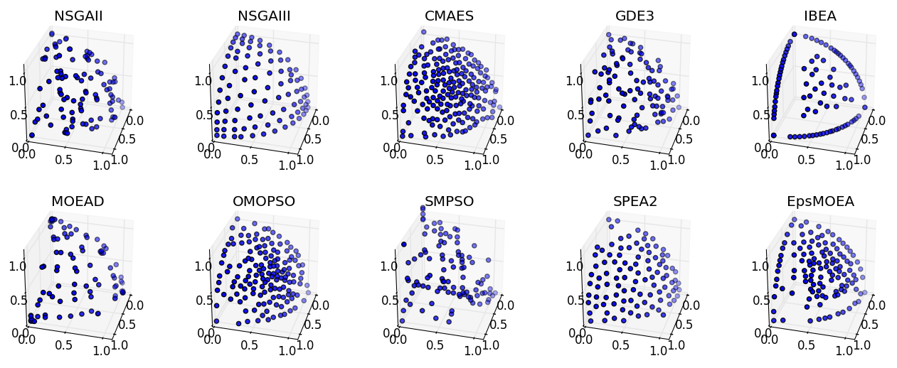
Comparing Algorithms Visually

Extending the previous examples, we can perform a full comparison of all supported algorithms on the DTLZ2 problem and display the results visually. Note that several algorithms, such as NSGA-III, CMAES, OMOPSO, and EpsMOEA, require additional parameters.

from platypus.algorithms import *
from platypus.problems import DTLZ2
from platypus.experimenter import experiment
from multiprocessing import Pool, freeze_support
import matplotlib.pyplot as plt
from mpl_toolkits.mplot3d import Axes3D

if __name__ == '__main__':
    freeze_support() # required on Windows
    pool = Pool(6)

    # setup the experiment
    problem = DTLZ2(3)
    algorithms = [NSGAII,
                  (NSGAIII, {"divisions":12}),
                  (CMAES, {"epsilons":[0.05]}),
                  GDE3,
                  IBEA,
                  MOEAD,
                  (OMOPSO, {"epsilons":[0.05]}),
                  SMPSO,
                  SPEA2,
                  (EpsMOEA, {"epsilons":[0.05]})]

    # run the experiment
    results = experiment(algorithms, problem, seeds=1, nfe=10000, map=pool.map)

    # display the results
    fig = plt.figure()

    for i, algorithm in enumerate(results.iterkeys()):
        result = results[algorithm]["DTLZ2"][0]

        ax = fig.add_subplot(2, 5, i+1, projection='3d')
        ax.scatter([s.objectives[0] for s in result],
                   [s.objectives[1] for s in result],
                   [s.objectives[2] for s in result])
        ax.set_title(algorithm)
        ax.set_xlim([0, 1.1])
        ax.set_ylim([0, 1.1])
        ax.set_zlim([0, 1.1])
        ax.view_init(elev=30.0, azim=15.0)
        ax.locator_params(nbins=4)

    plt.show()

    pool.close()
    pool.join()

Running this script produces the figure below: